SPC - Statistical Process Control; the Normal Distribution; Skewed Distributions; Process Capability Indices

Statistical Process Control (SPC) (Page 3 of 4)

The lower control limit LCL and the upper control limit UCL of a process may be calculated from the mean and standard deviation (or sigma) of the plotted data as follows:

LCL = Mean - (3 x Sigma);

UCL = Mean + (3 x Sigma).

Thus, the span from the LCL of a process to its UCL is 6 sigma. The probability of getting points outside this +/- 3 sigma range is already very low (see Table 1). Getting a measurement outside this range should therefore warn an engineer that something abnormal is happening, i.e., the process may be going out of control. This is the reason why these boundaries are known as 'control limits.'

LINKS:

Once the control limits have been included on the control charts (also in the form of horizontal lines like the specification limits), the operator can start using the chart visually to detect anomalous trends in the process that she would need to notify the engineer about.

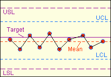
Figure 3. Example of a control chart showing data that are

slightly off-centered, but nonetheless in control and within specs

For instance, any measurement outside the control limits is an automatic cause for alarm, because the probability of getting such a measurement is low. Four (4) or more consecutively increasing or decreasing points form a trend that is not normal, and therefore deserves attention. Six (6) consecutive points on one side of the mean also deserve investigation. When such abnormalities are observed, the process owner must take an action to bring the process back to its normal behavior.

Control limits must be recomputed regularly (say, every quarter), to ensure that the control limits being used by the operator are reflective of the current process behavior.

Read more about: Control Charting.

The Process Capability Indices

Being able to monitor a process for out-of-control situations is one thing; knowing how a process actually performs is another. Eyeballing the centering and shape of a data distribution can give us quick, useful information on how the corresponding process behaves, but it is not very helpful in quantifying the process' actual and potential performance. It is for this reason that statisticians have come up with methods for expressing the behavior or capability of process distributions in terms of single numbers known as process capability indices.

Process capability refers to the ability of a process to meet customer requirements or specification limits, i.e., how consistent its output is in being within its lower and upper spec limits. A process capability index should therefore be able to indicate how well the process can meet its specs.

The most basic process capability index is known as the simple process capability index, denoted by 'Cp'. Cp quantifies the stability of a process, i.e., the consistency of its output. As mentioned earlier, the process capability indices discussed here presume the normality of the process. As such, the inconsistency of the process may be measured in terms of the standard deviation or sigma of the output data of the process. This is what Cp does - it uses the sigma to quantify the variation of a process, and compares it against the distance between the upper spec limit (USL) and lower spec limit (LSL) of the process. In mathematical form:

Cp = (USL - LSL) / (6 x Sigma)

The quantity (USL - LSL) is basically the range of output that the process must meet, while 6 sigma corresponds to +/- 3 sigma from the mean, or 99.73% of all the process output data. The smaller the value of 6 sigma, the narrower the process output distribution is, denoting higher stability. Thus, Cp increases as process stability increases. Thus, a process needs a Cp > 1 to ensure that it is narrow enough to meet the spec range 99.73% of the time.

HOME